Key Terms
- Isotope: a "species" of atom, differentiated from other isotopes of the same atom type by the number of neutrons.
- Isotopic fractionation: the unequal incorporation of isotopes of varying atomic weights during natural or laboratory processes.
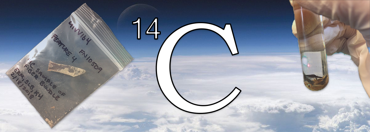
- Assay: (noun) results of an analysis of a material's components, or the material which has undergone this analysis; (verb) to investigate a sample of material to determine its contents—in the case of radiocarbon dating, carbon isotope quantities.
- Legacy date or assay: assays that have been obtained from older research projects. Legacy assays may have been pretreated, measured, or originally reported using antiquated methods or standards.
- Measured age: a radiocarbon age in its most raw form—it has not been adjusted to account for isotopic fractionation nor calibrated to be comparable to the modern solar calendar. Measured ages were commonly reported by radiocarbon labs prior to the late-1970s.
- Conventional age: a radiocarbon measurement corrected for isotopic fractionation but not calibrated. Conventional ages are reported by radiocarbon labs today. They adhere to published standards and are stated in radiocarbon years before present (RCYBP; years before AD 1950).
- Radiocarbon date: a conventional age which has been calibrated to correspond with our solar calendar, stated as calibrated years before present (cal BP), cal BC/AD, or or cal BCE/CE.
- Reservoir effect: a difference in carbon levels between an environment, usually a marine or freshwater system, which incorporates and stores carbon differently than the atmosphere.
- Targeted event: also called event of interest, this is the behavioral or natural event the archeologist is trying to date.
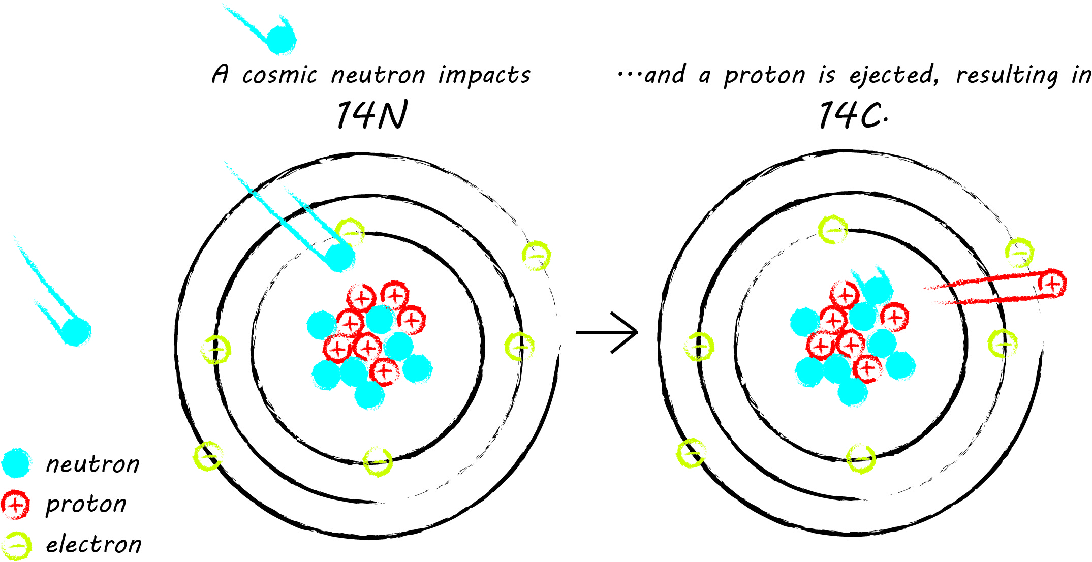
Radiocarbon is an unstable isotope of carbon, often written as carbon-14 or 14C. An isotope is a variety of atom, differentiated from other atoms of the same type by the number of neutrons in its nucleus. There are three naturally-occurring carbon isotopes: the stable isotopes 12C and 13C, and the unstable radiocarbon isotope. 14C has an atomic mass of 14, comprised of 6 protons and 8 neutrons (all carbon atoms have 6 protons). Most 14C is created in the upper atmosphere, where, on rare occasion, thermal neutrons from cosmic rays impact atmospheric nitrogen-14 (14N), resulting in the ejection of a proton from the nucleus of the nitrogen atom, which is replaced by the impacting neutron. Then, radiocarbon reacts with oxygen, producing carbon dioxide (CO2). The stable carbon isotopes undergo the same transformation to CO2. CO2 is then distributed throughout the earth's atmosphere and incorporated into living things through photosynthesis and the food chain.
When the radiocarbon dating method was in its infancy, scientists assumed that CO2 was evenly distributed in the atmosphere. This assumption proved false. Fortunately, the problem of irregular atmospheric mixing of carbon can be minimized by using radiocarbon calibration curves. Atmospheric mixing and calibration curves are discussed further in In the Environment.
After carbon isotopes are incorporated into plants through photosynthesis, they travel up the food chain from plants to animals. The radioactive decay of 14C (the random, spontaneous conversion of 14C back into 14N) is always occurring, regardless of whether an organism is alive or dead. While alive, organisms continue to take in carbon. Carbon levels remain in equilibrium with atmospheric levels due to metabolic processes in the plant or animal.
Once an organism is no longer participating in the carbon cycle through metabolic processes, due to death or other means (such as the seperation of fingernails and feathers), 14C returns to 14N through a type of radioactive decay called beta-decay. Beta-decay of 14C is caused by a neutron in 14C producing and ejecting an electron and an electron anti-neutrino, and ultimately transforming into a proton. Remember, 14C was created by a neutron colliding with 14N and replacing a proton in 14N with that neutron; during beta-decay the processes is reversed.
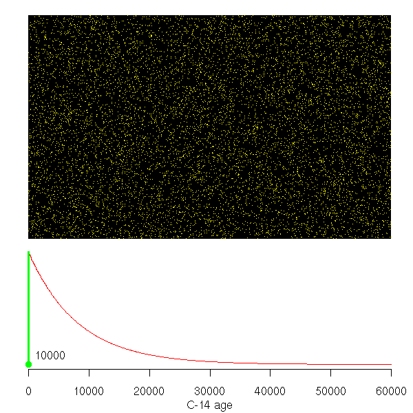
The decay rate of 14C is called its half-life—the amount of time it takes for half of a given quantity of 14C to transform back into 14N. The decay process is random—scientists cannot predict which specific atoms will decay in a given moment—but the decay rate is constant. Simply put, as radiocarbon decays, about half of the total quantity of 14C in the once-living sample will decay over the course of 5730 years. After twice that time has passed, 11,460 years, the 14C will have halved again (25% of the original quantity will remain after 11,460 years), and so on. By about 55,000 years, there will not be enough radiocarbon remaining to be detected with current measurement technologies.
Confusingly, the precise half-life of radiocarbon is not known. The half-life calculated by radiocarbon dating's inventor, Willard Libby, is known as the Libby half-life (5568 ± 30 years). The Libby half-life continues to be used to calculate radiocarbon ages despite more accurate half-life measurements that have been made since. While using the less-accurate Libby half-life sounds problematic, it is not! Radiocarbon ages are corrected using calibration curves which are also based on the Libby half-life, and consistency in the use of the Libby half-life allows for comparable measurements. An explanation of how calibration curves are built and used, below, will make this concept more understandable.
Several methods of measuring 14C have been used over the decades. Today, most radiocarbon measurements are made by Accelerator Mass Spectrometry (AMS). Before AMS was developed, measurements were made by liquid scintillation spectrometry, gas proportional counting, and, in radiocarbon dating's infancy, Geiger counters. Conventional methods, as these are known, count 14C decay in real time. The chief drawback to conventional methods is that they require a relatively large sample of material. For wood charcoal, an entire handful of charcoal chunks was typically submitted for a single assay. Bone required about 300 grams of sample material, and early assays on ivory or teeth required as much as five pounds of sample material! Dating by AMS, which measures the ratio of 14C to one of the stable carbon isotopes (12C, 13C), uses much smaller samples, as small as a single grain of rice or even less. In AMS dating, the original quantity of 14C (the amount at death of the organism) is estimated by comparing the measured quantity of 14C to the quantity of the stable carbon isotopes. Then, the Libby half-life is used to calculate how much time has passed since the original quantity of 14C decayed into the measured quantity of 14C.
Age versus Date
The radiocarbon age is not the same as the radiocarbon date; this is because the radiocarbon calendar is not the same as our annual (solar) calendar. Calibration curves are needed to calculate the calendar date based on the radiocarbon age. It is also important to remember that both radiocarbon dates and radiocarbon ages are estimated ranges of possible dates.
For example, if the laboratory measured age is 4000 ± 30 RCYBP, it is not necessarily more likely that the radiocarbon dated event occurred in 4000 RCYBP than anywhere else in the probability range.
The radiocarbon age is given in radiocarbon years before present (RCYBP, or sometimes BP). "Present" is the year AD 1950, when the radiocarbon dating method was unveiled. Even though our "present" changes every day, the radiocarbon dating "Present" of AD 1950 is frozen in time. Typically, a radiocarbon age is reported as a mean and standard error, like this:
mean ± standard error
For example: 4000 ± 30 RCYBP is equivalent to 4030-3970 RCYBP
As mentioned, early radiocarbon scientists assumed that the ratio of atmospheric carbon (12C, 13C, and 14C) was the same around the planet at any given time. However, it was not long before they realized that ratios of atmospheric carbon do, in fact, vary through time and across space. Quantities and distribution of atmospheric radiocarbon are affected by the earth's magnetic field, solar flares, major volcanic eruptions, and, in more recent centuries, by the burning of fossil fuels and nuclear detonations. Their influences are reflected in the quantity of carbon in the materials we date.
The burning of fossil fuels during the industrial revolution released ancient carbon into the atmosphere; this carbon is so old that it contains little 14C, so it dilutes the ratios of 14C to the stable carbon isotopes found in the atmosphere. During the atomic age (1940s-1960s), on the other hand, nuclear detonations released neutrons which resulted in the creation of large quantities of 14C.
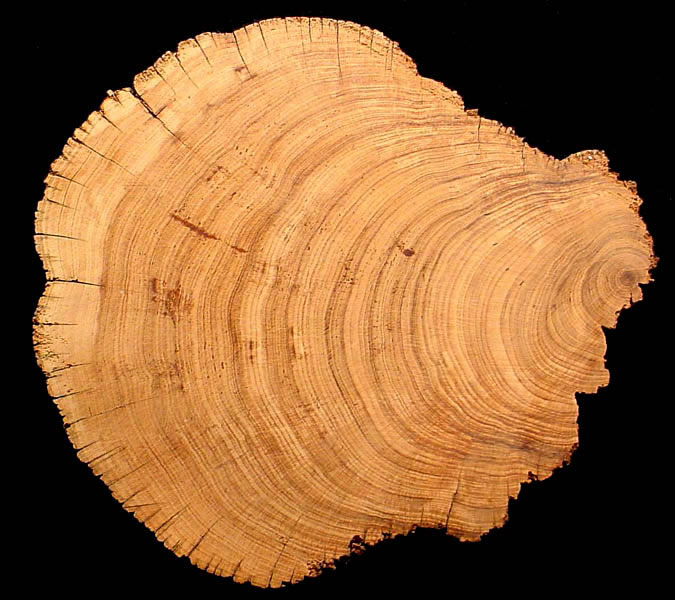
Differences in atmospheric carbon are corrected for using a calibration curve. Tree ring sequences were used to generate much of the calibration curve that we use today and are considered proxy records for past carbon quantities. Other proxy records used to construct calibration curves include sea corals and varves (layered lake sediments). Consider that tree rings grow annually and reflect the environmental conditions in which they live. In wet years, trees typically grow faster and the annual growth rings are thicker; in dry years or when the tree is stressed, the rings are thinner. Dendrochronologists, the scientists who study tree-rings, create databases of tree ring sequences that go back thousands of years! Because sequenced tree rings can be simply counted to derive an age for the tree and rings of known age can be radiocarbon dated, fluctuations in atmospheric radiocarbon can be correlated with a precisely counted calendar year. If you graph the relationship between known years (the date) on one axis and carbon ratios (the radiocarbon age) on the other axis, then you have a calibration curve.
Interestingly, carbon levels vary around the world as well. Because of differences in carbon ratios in the northern and southern hemispheres, each has its own calibration curve. A marine curve has also been developed, because the ocean stores carbon differently than the atmosphere—this is an example of a reservoir effect. Carbon ratios can vary between marine environments as well, due to currents and differential mixing of surface and deep waters. Areas of coastal upwelling, where deep ocean waters are brought to the surface due to currents and ocean floor topography, are locations where marine carbon reservoirs will likely be unique. In such cases, radiocarbon ages may require a local reservoir correction. Freshwater systems also may require reservoir corrections.
Importantly, calibration curves change through time as new information is incorporated. Updated calibration curves are released periodically. Fortunately, new calibrations curves do not render radiocarbon assays made decades ago irrelevant—the radiocarbon age can simply be recalibrated with new curves. Once an age is calibrated it is known as a date. Calibrated radiocarbon dates are typically given as a date range expressed as either "cal BC/AD" or "cal BP," with "cal" standing for "calibrated" and "calendar."
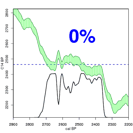
How the calibration curve and radiocarbon age are used to calculate a radiocarbon date is not complex, but it can be difficult to describe. The animations below are helpful illustrations of the concept. Recall that a radiocarbon age is given as a date range. Statistically speaking, this date range has a normal distribution (the bell curve on the left side of the first animation). However, when the radiocarbon date is calculated using the calibration curve (the green area), the resulting probability distribution is not normally distributed (it is not a symmetrical bell-shaped distribution). Look at the black line that is created on the bottom of the animation as the blue dashed lines link where the green calibration curve intersects with the timeline represented by the bell curve on the left. The black line on the bottom of the animation has many dips and spikes—it is not a normal distribution.
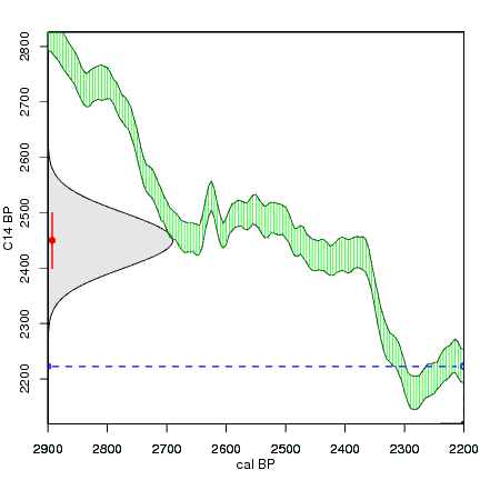
The next animation illustrates the concept of the likelihood that of the true date falling within a given date range. Let's pretend that the radiocarbon assay was made on a juniper berry. The date of death for the berry would be the day it was picked or fell off the plant. The animated distribution below is the same as the one generated in the animation above. Note the x-axis is years cal BP (calibrated years before present)—you can ignore the y-axis now. Watch as the blue dashed line crosses the black distribution outline and colors sections under the high humps gray. As the gray areas increase in size, the percentage of likelihood that the true date falls within the gray area increases. This should make it obvious that the true date may fall anywhere under the distribution. However, it is more likely that it will fall under high areas of the distribution than low ones. Because radiocarbon date ranges often span several centuries, it is useful for the archeologist to narrow the date ranges to areas of high probability. In publications, it is standard to report radiocarbon dates as a likelihood, or confidence level, of 95% (2σ, also written 2-sigma) or 68% (1σ). Don't worry about doing these calculations by hand—radiocarbon calibration programs like OxCal will do them for you.
101 Summarized
Most 14C is created in the atmosphere. It is incorporated into plants via photosynthesis and animals via the food they eat. Radiocarbon measurements can be made on organic (once living) materials that are younger than 55,000 years. Upon death of the organism, unstable 14C decays without replenishment. The radiocarbon age is a calculation based on the amount of 14C left in a sample and the radiocarbon half-life. The radiocarbon age requires adjustment using a calibration curve to become a meaningful date in our solar calendrical system.
Other sections in the exhibit expand on topics introduced here: In the Environment discusses how radiocarbon behaves in the environment, In The Lab lifts the curtain on what happens behind the scenes in an accelerator mass spectrometry (AMS) radiocarbon dating lab, and In Libby's Test Tube details the intriguing history of radiocarbon dating. Together, these sections lay essential groundwork for understanding of radiocarbon dating in the 21st century. But it does not end there.
To implement a radiocarbon dating program for an archeological site or region, the archeologist must know how to choose appropriate dating materials, covered in Selecting Samples, how to properly report radiocarbon data, discussed in Reporting Results, and how to relate the radiocarbon date to the archeological problem it is intended to address, presented in Interpreting Radiocarbon Results. A Case Study from the Lower Pecos Canyonlands shows how a large radiocarbon dataset can be used to investigate a diversity of archeological questions, and Radiocarbon Takeaways summarizes important points for future radiocarbon endeavors!