On this page:
This section explores how radiocarbon (14C) behaves in nature—the atmosphere, terrestrial and marine environments, and at the organismal level—and outlines methods used by radiocarbon scientists to adjust for differences in radiocarbon behavior across time and space.
Up in the Atmosphere: Cosmic Origins
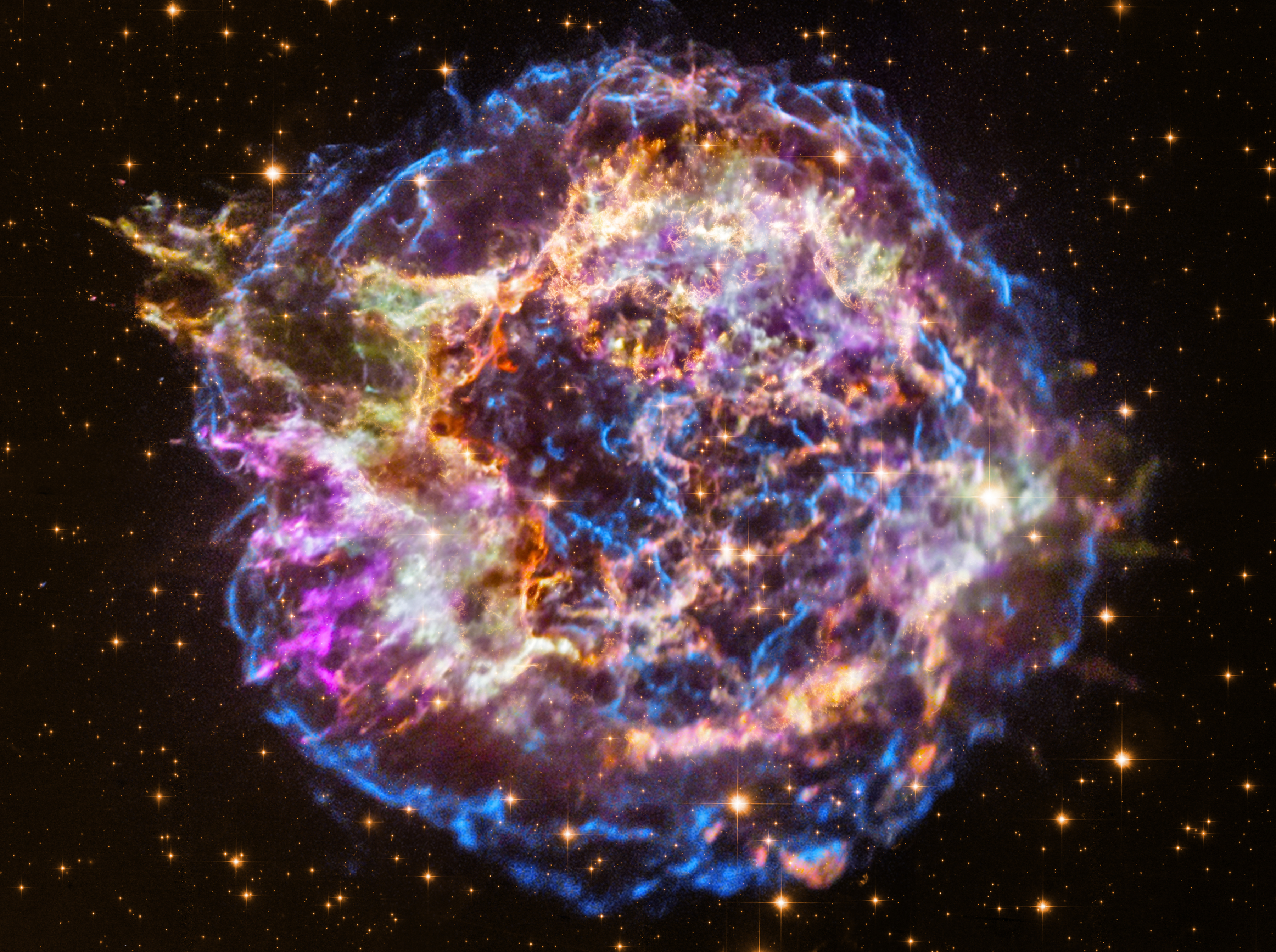
Most 14C is created in the earth’s upper atmosphere when thermal neutrons from cosmic rays react with nitrogen-14 (14N). Cosmic rays are generated by the sun as well as by activity outside the solar system, such as supernovae. The abundance of cosmic particles impacting earth's atmosphere and the deflection of some of these particles by earth's magnetic field relates directly to how much 14C is created at a given time. Therefore, the amount of 14C created varies through time.
Cosmic rays are comprised of subatomic particles: electrons, protons, and, most importantly for the creation of radiocarbon, neutrons. When cosmic neutrons collide with 14N they sometimes cause the nitrogen isotope to eject a proton which is then replaced with the offending neutron. The result of the exchange is the creation of 14C. Radiocarbon then reacts with oxygen to become carbon dioxide (CO2) (the other carbon isotopes also do this). Stratospheric and tropospheric winds distribute the 14CO2 (and 12CO2 and 13CO2) throughout the atmosphere.
The cosmic exchanges creating 14C are rare, and so 14C comprises a tiny fraction of all carbon—far less than 1% (specifically, 10-12%). The most abundant carbon isotope is 12C, comprising over 98% of natural carbon. The atomic weight of an isotope is the sum of its protons and neutrons—symbolized as the superscript number before the elemental letter. All three carbon isotopes have six protons so, as you might have deduced, it is their neutron count that differs. The three carbon isotopes behave similarly, chemically speaking. However, their different weights can have a small but measurable effect on their physical behavior, which results in isotopic fractionation. In radiocarbon dating, isotopic fractionation results from the discriminatory incorporation of isotopes of varying atomic weights during natural process (such as photosynthesis) or laboratory processes.
Calibrating for Change: Calibration Curves
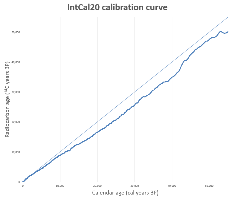
As noted, the quantity of atmospheric carbon created varies through time. It also varies geographically as the result of earth's complex natural systems. Radiocarbon calibration curves serve to correct for these differences across time and space, and correlate radiocarbon time with our solar calendar. New calibration curves are published periodically as scientists gather more data. But wait! Does this mean that calibration curves will become outdated as new, better curves are created? Yes, they do. Radiocarbon ages need to be re-calibrated as calibration curves are updated, at least when new analyses are undertaken using old radiocarbon data. Think of the ongoing revision of calibration curves not as a chaotic restructuring of time, but as closer and closer statistical approximation of the event of interest (the date).
The most recent calibration curves were finalized in 2020: a Northern Hemisphere curve (IntCal20), a southern Hemisphere curve (SHCal20), and a baseline global marine reservoir curve (Marine20). A single global curve does not exist because global carbon distributions are affected by natural patterns such as winds, ocean upwelling, and land-to-water ratios.
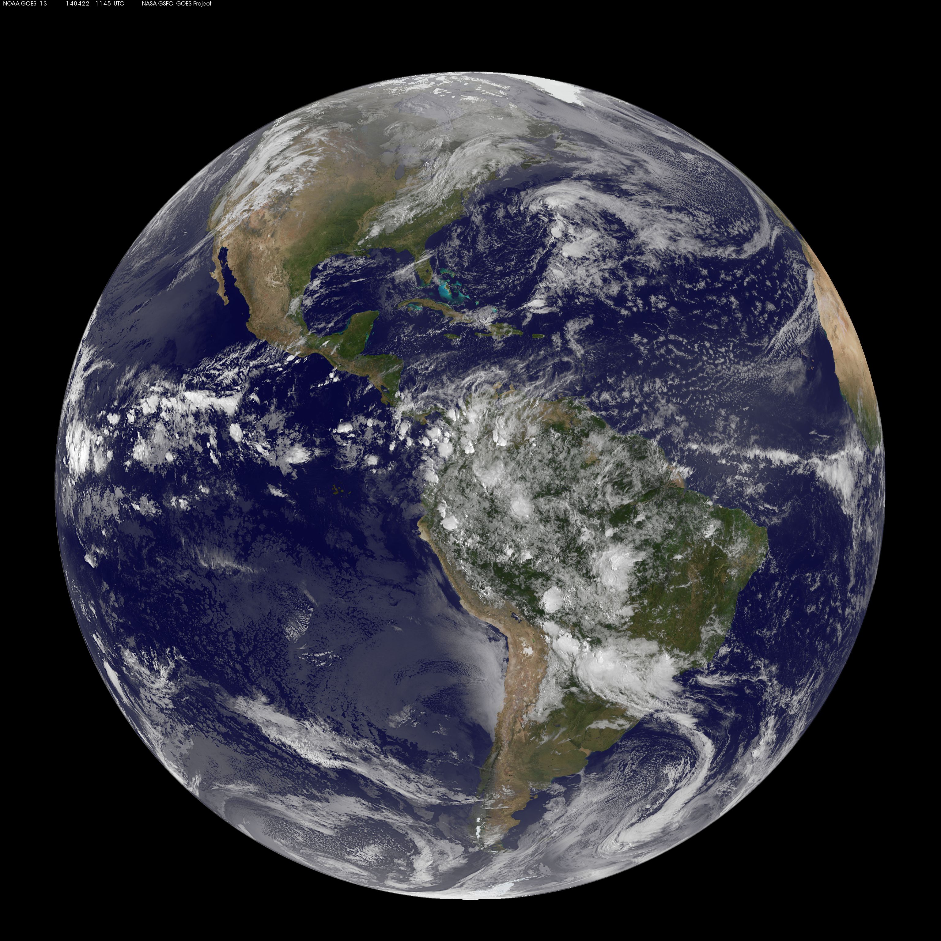
The hemisphere curves correlate with the atmospheric hemispheres, which are slightly different than the geographic northern and southern hemispheres neatly divided by the equator. Complex atmospheric mixing in the equatorial region due to winds at the Intertropical Convergence Zone cause carbon variability as well. In equatorial regions the geographic southern hemisphere may be better represented by the northern hemisphere curve, and vice versa. It is possible to mix the curves in calibration programs such as OxCal, if this can be justified by the geographic origin of the radiocarbon sample. Both the northern and southern hemisphere curves are most accurate for mid-latitudes and less reliable for high latitudes or great altitudes.
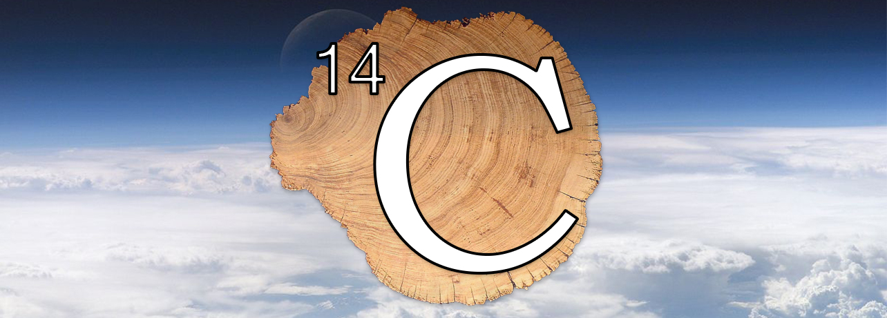
Sample materials used as proxies for past atmospheric conditions (also called “archives") include tree rings, corals, foraminifera (single-celled animal plankton), and speleothems (mineral cave deposits). Trees are one of nature’s great timekeepers; their ages can be determined through the study of annual growth rings—dendrochronology. Dendrochronological sequences were the first carbon proxy used to construct a calibration curve, and remain the preferred proxy record. Because the age of a tree ring can be determined by both radiocarbon dating and by counting, the difference between the radiocarbon age and the true age can be calculated and used to adjust the ages of other materials that perished the same year the tree ring grew.
The IntCal20 curve includes European oak and pine chronologies, the North American bristlecone pine chronology, Japanese chronologies, and several "floating" European chronologies, which have been anchored by wiggle-matching. Wiggle-matching is used to refine the calibrated date of a radiocarbon measurement that falls within a plateau in the calibration curve, by matching the curve of the calibrated date with the small wiggles found on the calibration curve. Typically, this method is undertaken for a series of radiocarbon dates with known differences in age (for example, radiocarbon Sample X is known to be 45 years older than Sample Y), the kind of information that is typically only available for dated materials like a related series of tree rings, which can be counted. Together, these dendrochronologies span the last 14,200 years (cal BP) of the Intcal20 curve.
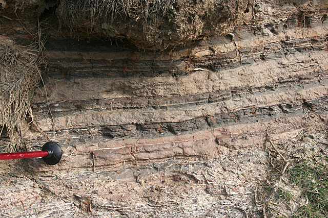
Scientists also use pollen grains, leaves, and other terrestrial macrofossils from unmixed, varved sediments (annually deposited stratigraphic layers >1cm thick) to establish independent carbon time scales. The IntCal20 curve uses macrofossils from varved sediments from Lake Suigetsu in Japan to extend the radiocarbon time scale back to ca. 55,000 cal BP.
Scientists strengthen problematic areas of the calibration curve—those with insufficient or contradictory data—with chronologies from non-varved marine foraminifera and uranium-thorium dated aragonitic corals and speleothems. Corals and foraminifera reflect both atmospheric and marine reservoir carbon sources, called the mixed marine layer. Speleothems incorporate fossil carbon (carbon so old that all the 14C has decayed), which is corrected for by comparing overlapping speleothem records with varved macro-fossil and dendrochronological records to ascertain a constant background value of this inert carbon.
In sum, radiocarbon calibration curves are a work-in-progress being refined over time, much like the archaeological chronologies that rely upon them.
Surf and Turf: Reservoir Effects
As discussed above, calibration curves are based on proxies for atmospheric carbon levels. But what if you want to radiocarbon date something that takes in carbon from sources other than the atmosphere, such as aquatic environments, or places that have different carbon levels due to nearby phenomena like active volcanism? Organisms that lived in these environments have quantities of carbon that differ from the atmosphere. Simply put, when radiocarbon dated, they are likely to yield an incorrect date. This is called the reservoir effect. While dating materials that intake carbon from other sources, or reservoirs as they are known, presents challenges, there are methods for adjusting their ages to make them more accurate.
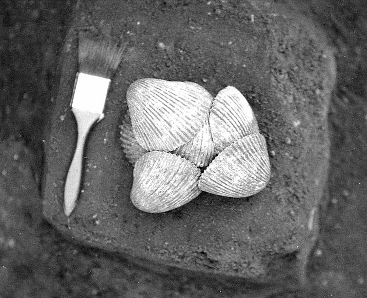
Marine (saltwater) and freshwater (also called hardwater) reservoir effects are probably the most-common types of reservoir effects archeologists encounter. Aquatic plants and animals engage in a complex carbon exchange network, taking in dissolved fossil carbon (carbon-bearing material in which all 14C has decayed) from rivers, oceans, or lakes, as well as atmospheric carbon that is mixed into aquatic systems through natural processes. Typically, the radiocarbon age of the aquatic organism will measure older than contemporaneous terrestrial plants and animals. Interestingly, terrestrial animals that eat from aquatic reservoirs, such as fishing birds and even people who eat a lot of fish, also reflect aquatic reservoir effects when radiocarbon dated. The Marine20 calibration curve provides a baseline for correcting marine assays, but samples from unique marine environmental conditions may require further adjustments.
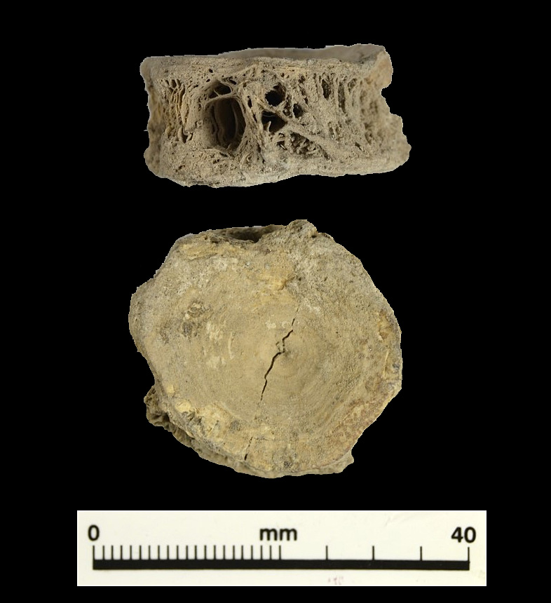
Freshwater or hardwater reservoir effects can be more difficult to adjust for than marine reservoir effects. Hardwater effects result from the presence of dissolved carbon from geologic deposits like limestone, which are common in parts of Texas. Made from marine organisms that accumulated on the sea floor millions of years ago, the 14C in limestone has fully decayed and only the stable carbon isotopes 12C and 13C persist (fossil or dead carbon). When a living organism, such as a catfish in the Pecos River, uptakes fossil carbon from its environment, the carbon in the fish is not in equilibrium with atmospheric carbon. Hardwater reservoir effects are particularly difficult to account for because carbon levels in rivers fluctuate seasonally, and radiocarbon quantities may lie anywhere between atmospheric and bedrock levels. These effects have been shown to cause radiocarbon ages to be as much as 800 years too old!
While not technically a hardwater effect, the influence of limestone on Texas fauna is also seen in terrestrial gastropod (snail) ages, which have been shown to be hundreds of years too old! Why? Gastropods sometimes incorporate fossil carbon from limestone into their shells.
To correct for marine reservoir effects, archeologists use the Marine20 calibration curve (where appropriate), or calculate a ∆R (Delta R) value to adjust conventional ages for reservoir effects. The value can be estimated by dating closely associated archeological samples of different material types (for example, marine and terrestrial), by comparing dates on modern terrestrial and aquatic samples, or by dating correlated volcanic tephra deposits from terrestrial and marine environments.
A Heavy Load: Isotopic Fractionation
The distinct atomic weights of the three carbon isotopes (that is, 12C, 13C, and 14C) cause the isotopes to behave slightly differently from each other in certain processes—this is called fractionation. Isotopic fractionation in radiocarbon dating takes two forms: fractionation due to natural processes and fractionation that occurs during sample pretreatment and measurement by accelerator mass spectrometer (AMS).
Isotopic fractionation is quantified as a delta-13C (δ13C) value, which is a ratio of 12C to 13C as compared to a known standard (the Pee Dee Belemnite limestone formation, or PDB), in parts per thousand (per mille). The more negative the δ13C, the greater abundance of 12C compared to the heavier carbon isotopes.
Photosynthesis is the primary mechanism of natural fractionation of carbon isotopes. Lighter carbon isotopes are differentially incorporated into the plant during respiration and internal chemical processes. As a result, plant carbon ratios are different than atmospheric carbon ratios. This effect is transferred up the food chain.
Photosynthetic Pathways
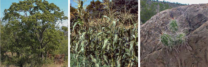
There are three photosynthetic pathways: C3, C4, and crassulacean acid metabolism (CAM). Why is understanding this important? Before modern standards in radiocarbon dating were established, most radiocarbon ages were not adjusted for isotopic fractionation. Archeologists who want to use this uncorrected data today must correct the legacy dates with an estimate of the natural isotopic fractionation value (the delta-13C; δ13C). Understanding that different photosynthetic pathways exist can aid archeologists in using an accurate estimate.The photosynthetic pathways reflect plant adaptations for temperature, moisture, and atmospheric abundance of CO2. C3 plants are the most common plant type globally, and include trees and shrubs which prefer cooler, higher CO2 environments. C4 plants include many warm season grasses, such as corn and sugar cane, and make up an estimated 18% of plants globally, and are adapted for hotter, lower CO2 environments. CAM plants include most succulents, including cacti, and many evergreen rosettes such as agave and yucca. While CAM plants comprise the smallest percentage of plants globally, they are abundant in many parts of Texas. Adapted to arid environments, CAM plants switch between photosynthetic pathways as environmental conditions dictate. During the daytime, CAM plants generally employ a C3 photosynthetic pathway, and at night employ a process similar to C4.
The δ13C value of a sample can be measured one of two ways—during AMS measurement or by isotope ratio mass spectrometry (IRMS). The AMS δ13C measurement includes both isotopic fractionation that occurs due to natural processes and fractionation which occurs during laboratory processing. The AMS δ13C is the value used to correct the measured radiocarbon age (making it a conventional radiocarbon age—see Reporting Results). In contrast, the IRMS δ13C only measures natural isotopic fractionation; this value is commonly used for investigating diet (such as that of ancient humans), but it is, emphatically, not used for correcting radiocarbon ages measured by AMS. Radiocarbon dates measured by conventional methods (not AMS), such as legacy dates, the IRMS δ13C can be used to adjust the radiocarbon age in much the same way as an AMS δ13C measurement.